Expected number of non-uniform draws until collision?

Question

Edit May 9 -- high-level summary of the issue here. $R$ gives a good proxy for estimating collision time, with a slight undercount. Random matrices and graphs give distributions with longer time until collision than what you'd expect by looking at their values of $R$

Suppose I do IID draws from multinomial distribution with probabilities $p_1,\ldots,p_n$. Is there a nice approximation for the $x(p)$, the expected number of draws from $p$ until collision, ie, drawing some $i$ more than once?

In the case of $p_1=p_2=\dots=p_n$, this was shown to be the following

$$x(p)=\sqrt{\frac{\pi n}{2}}$$

---

From simulations, the following appears to be a lower bound

$$x(p)\approx \sqrt{\frac{\pi R}{2}}$$

where $R=\frac{1}{\|p\|^2}$ and $\|p\|^2=p_1^2+\ldots+p_n^2$ is the probability of observing a collision in two IID draws from $p$.

Distributions were taken to be of the form $p_i\propto i^{-c}$ with $c$ varying

Answer 1

An approximation

Let $X_i$ ($i=1,2 \cdots $) be the result of $i-$th draw, let $C_{i,j}\equiv X_i = X_j$ ($i<j)$ be the colission event for the pair $(i,j)$. Let the event $D_k = \cap_{i<j\le k} C_{i,j}$ correspond to having all first $k$ draws different (no collisions); let $d_k = P(D_k)$. Clearly, $d_1=1$ , $d_{n+1}=0$.

Let $F_k$ be the event of having our first collision at draw $k$, and let $f_k=P(F_k)$

Then $$\begin{align} f_k &=\sum_{i=1}^{k-1} P(X_k = X_i\cap D_{k-1}) \\ &= P(D_{k-1})\sum_{i=1}^{k-1} P(X_k = X_i | D_{k-1}) \\ &= d_{k-1} \, (k-1) P(X_k = X_1 | D_{k-1}) \\ \tag{1} & \approx d_{k-1} \, (k-1) P(X_k = X_1 ) \\ &= d_{k-1} \, (k-1) \, \alpha \\ \end{align}$$

where $\alpha = \sum_{m=1}^n p_m^2$. We have $f_1=0$ and $f_2 = \alpha$.

Also: $$\begin{align} d_k &= d_{k-1} -f_k \\ \tag{2} \end{align}$$

This system is solved by

$$ d_k = \prod_{j=1}^{k-1} (1- j \alpha) \\ \tag{3}$$

(Actually, we need to truncate the product so that $d_k \ge 0$)

Finally, the expected time for next colission would be $$x(p) = 2 + \sum_{k=2}^n d_k = 2 + \sum_{k=2}^n \prod_{j=1}^{\min(k-1,1/\alpha)} (1- j \alpha)$$

Update: This approach does not seem promising. Actually $P(X_k = X_1 | D_{k-1}) \approx \alpha$ is only valid near $k=2$ ; at the other extreme $P(X_{n+1} = X_1 | D_{n}) = 1/n$.

Alternatively, one might resort to Newton's identities, noticing that our $d_k$ correspond to $ k! e_k$ in that page. This allows to compute $d_k$ (and hence $x(p)$) numerically, from $\alpha$ and the other power sums (which correspond to $p_k$ there) - as in JimB's answer. But, again, this does not seem to provide much insight about the asymptotics or approximations.

---

Added: another way to get the numerical exact solution, probably useless (numerically unstable), using Poissonization and numerical depoissonization.

Matlab/Octave code:

n = 20
c = 1  % constant for p(i) = i^(-c)
pp = [1:n].^(-c); % probabilities
pp = pp/sum(pp);  % normalized
POI = zeros(n+1); % Poisson transform matrix
for i = 0:n
 for j = 0:n
  POI(i+1,j+1) = exp(-i)*(i)^(j)/factorial(j);
 endfor
endfor
% prob of no collision, for the Poisson model
gk=zeros(n+1,1); 
for k=0:n
   gk(k+1) = exp(-k) * prod(1+k*pp);
endfor
% prob of no collision, for the multinomial (exact) model
dk = linsolve(POI,gk) ;
%expected time
sum(dk)

This gives $x(p) = 4.6333757$

---

Answer 2

Edit: At the end I've added a Mathematica function that will calculate the complete distribution rather than just the mean. Depending on the options selected, one can find the "exact" distribution or the "approximately exact" distribution which depends on using machine precision numbers which results in a considerable increase in speed.

Original answer:

One can find the exact mean. Using Mathematica below is code that produces simulations from a multinomial to estimate the mean and the exact formula for the mean.

(* Generate 20 probabilities that sum to 1 *)
n = 20;
c = 1;
p = Table[i^(-c), {i, 20}];
p = p/Total[p];
(* Run simulations )
nsim = 1000000;
s[i_] := Sum[p[[j]]^i, {j, Length[p]}]
x = RandomChoice[p -> Range[Length[p]], {nsim, n + 1}];
mean = 0;
Do[k = 2;
 While[Select[x[[i, 1 ;; k - 1]], # == x[[i, k]] &] == {} && k < (n + 1), k = k + 1];
 mean = mean + k,
 {i, nsim}]
mean = mean/nsim // N
( 4.63702 *)
(* Exact mean )
kmax = Length[p] + 1;
2 s[2] + Sum[k (k - 1) MomentConvert[AugmentedSymmetricPolynomial[Join[{2}, ConstantArray[1, k - 2]]], 
  "PowerSymmetricPolynomial"], {k, 3, kmax}] /. 
   PowerSymmetricPolynomial[i_] -> s[i] // Expand // N
( 4.63338 *)

Revised answer:

The following function can find the exact distribution of the time until the first collision or the exact probabilities for a specific number of draws until the first collision happening up to 50 draws or the approximate probabilities when using machine precision numbers.

approxExact[d_, p_, OptionsPattern[]] := Module[{s, pr, prob, total,  kk},
  (* Returns the probability distribution of the number of draws until the first collision *)
  (* d is the number of multinomial classes *)
  (* The probability of selecting class i is proportional to i^(-p) *)
  (* Optional arguments: *)
  (* "epsilon" Continue until the total probability of events is at least 1-epsilon *)
  (* (default is 10^-8) *)
  (* "precision" Numeric precision of power symmetric polynomials (default is 50) *)
  (* "print" True or False to print results as one goes along (default is True) *)
  (* "kmax" Maximum order of power symmetric polynomials to consider (default is 50) *)
  s[k_] := N[HarmonicNumber[d, p k]/HarmonicNumber[d, p]^k, OptionValue["precision"]];
  pr = ConstantArray[{0, 0}, Min[d + 1, OptionValue["kmax"]]];
  pr[[All, 1]] = Range[Length[pr]];
  prob = MomentConvert[AugmentedSymmetricPolynomial[{2}],
    "PowerSymmetricPolynomial"] /. PowerSymmetricPolynomial[kk_] -> s[kk];
  pr[[1]] = {1, 0};
  pr[[2]] = {2, prob};
  total = prob;
  k = 2;
  If[OptionValue["print"], Print[{pr[[2]], total}]];
  While[total <= 1 - Rationalize[OptionValue["epsilon"], 0] && 
    k < OptionValue["kmax"] && k < d + 1, k = k + 1;
    pr[[k]] = {k, (k - 1) MomentConvert[AugmentedSymmetricPolynomial[ Join[{2}, ConstantArray[1, k - 2]]], 
        "PowerSymmetricPolynomial"] /. PowerSymmetricPolynomial[kk_] -> s[kk]};
    total = total + pr[[k, 2]];
   If[OptionValue["print"], Print[{pr[[k]], total}]]];
  pr[[2 ;; k]]]
Options[approxExact] = {"epsilon" -> 10^-6, "kmax" -> 50, "precision" -> 50, "print" -> False};

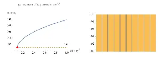
Consider $d=10$ and $p=1$:

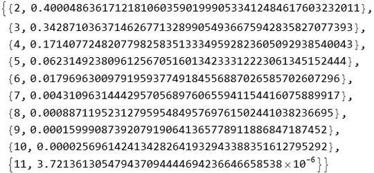
pmf1 = approxExact[10, 1]
(* {{2, 0.18064971668708334183046614833146934843581750460511},
    {3, 0.2659818277978277078742270573248618320164719105871},
    {4, 0.246306767894317825602528447941221519590155694619},
    {5, 0.168680227553142139284552160368127823227998051874},
    {6, 0.08880058815526647151857056458703230730218624454},
    {7, 0.03594943992243974232191051449091169926341719537},
    {8, 0.0109236474431937688476826236147190848157714520},
    {9, 0.0023611030135141392096358410495732957730522974},\
    {10, 0.000325160983801715352471323634201073447003952},
    {11, 0.000021520549413148157955318657882016128125697}}  *)
mean1 = pmf1[[All, 1]] . pmf1[[All, 2]]
(* 3.8844501770480480184116903511442503784417661 *)

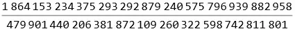
Now getting the exact values:

pmf2 = approxExact[10, 1, "epsilon" -> 0, "precision" -> ∞]

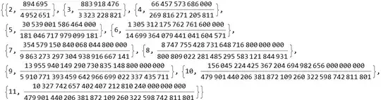
mean2 = pmf2[[All, 1]] . pmf2[[All, 2]]

This can even work for very large values of $d$:

pmf3 = approxExact[10000, 2]

The covers most of the probability distribution in that the sum of the probabilities shown above is 0.999999442316189999555627433782474244630006:

Total[pmf3[[All, 2]]]
(* 0.999999442316189999555627433782474244630006 *)

Answer 3

A possible explanation for your empirical approximation $\sqrt{\frac{\pi}{2 \sum p_i^2}}$

Let $d_k$ be the probability that there are no collisions in $k$ draws.

Then $d_1=1$ and $d_2 = \beta = 1- \alpha = 1-\sum p_i^2$

Now, for $k>2$ we can approximate $$d_k \approx \beta^{\frac12 k (k-1)} \tag 4$$

... assuming the probability that all pairs are distinct are approximately independent for $k \ll n$ - and because we expect $d_k$ to be relevant only in that range.

Here's an example (exact vs approximation), for $n=20$ , $p_i \propto 1/i$

Under this approximation, the expected number of draws time is given by

$$x(p) = \sum_{k=0}^\infty d_k = 1+ \sum_{k=1}^n d_k \approx 1 + \sum_{k=1}^n \beta^{\frac12 k (k-1)} \tag 5$$

Now $$\beta^{\frac12 k (k-1)} = \frac{1}{\beta^{1/8}} \exp\left( -\frac12 \frac{(k-\frac12)^2}{\sigma^2}\right)$$

where $\sigma^2 = -1/\log(\beta)$. The sum then can be approximated by a gaussian integral, so

$$x(p) \approx 1 + \sqrt{\frac{\pi}{2}} \sqrt{\frac{1}{-\beta^{1/4}\log \beta}} \tag 6$$

In our example, with $\alpha = 0.1233155$, this gives $x(p) \approx 4.512$ (against the exact $4.6333757$)

For large $n$, we expect $\alpha$ to be small. In that range,

$$x(p) \approx 1 + \sqrt{\frac{\pi}{2 \alpha}} + O(\alpha) \tag 7$$

In particular, in the equiprobable case $\alpha = 1/n$ and we recover the right asymptotics.

It's difficult to assert, however, if the approximation $(5)$ is asympotically correct, in some sense.