How to solve the system of nonlinear equations in N-R method or other numerical methods?

Question

Consider the system of infinite series \begin{align} &F=x+\frac{y^{3^2}}{3}+\frac{x^{3^5}}{3^2}+\frac{y^{3^7}}{3^3}+\frac{x^{3^{10}}}{3^4}+\frac{y^{3^{12}}}{3^5}+\cdots=0 \\ &G=y+\frac{x^{3^3}}{3}+\frac{y^{3^5}}{3^2}+\frac{x^{3^{8}}}{3^3}+\frac{y^{3^{10}}}{3^4}+\frac{y^{3^{13}}}{3^5}+\cdots=0. \end{align}

I want to approximate its zeros using Newton-Raphson process/ any other method.

Since the above system consists of infinite series, we don't have technique unless we truncate the system. I am considering the following truncated system \begin{align} &F(x,y)=x+\frac{y^{3^2}}{3}+\frac{x^{3^5}}{3^2}+\frac{y^{3^7}}{3^3}+\frac{x^{3^{10}}}{3^4}=0 \\ &G(x,y)=y+\frac{x^{3^3}}{3}+\frac{y^{3^5}}{3^2}+\frac{x^{3^{8}}}{3^3}+\frac{y^{3^{10}}}{3^4}=0. \end{align}

This one I am going to try at first.

---

Now in my previous post, I have asked to solve the following system \begin{align} &f(x,y)=x+\frac{y^{2^2}}{2}+\frac{x^{2^5}}{2^2}+\frac{y^{2^7}}{2^3}=0 \\ &g(x,y)=y+\frac{x^{2^3}}{2}+\frac{y^{2^5}}{2^2}+\frac{x^{2^8}}{2^3}=0. \end{align} The Sage code, given by the use @dan_fulea, was

IR = RealField(150)
var('x,y');
f = x + y^4/2 + x^32/4 + y^128/8
g = y + x^4/2 + y^32/4 + x^256/8
a, b = IR(-1), IR(-1)
J = matrix(2, 2, [diff(f, x), diff(f, y), diff(g, x), diff(g, y)])
v = vector(IR, 2, [IR(a), IR(b)])
for k in range(9):
    a, b = v[0], v[1]
    fv, gv = f.subs({x : a, y : b}), g.subs({x : a, y : b})
    print(f'x{k} = {a}\ny{k} = {b}')
    print(f'f(x{k}, y{k}) = {fv}\ng(x{k}, y{k}) = {gv}\n')
    v = v - J.subs({x : a, y : b}).inverse() * vector(IR, 2, [fv, gv])

Using the initial guess $(-1,-1)$, the N-R process converges at $8$th iteration.

---

Unfortunately the same code seems to be inefficient to solve the above truncated system $$F(x,y)=0=G(x,y).$$ It seems this system is associated with higher degrees and that is why the above code is efficient. It needs modification.

Is there a more efficient computer code to solve the above truncated system system in N-R method or other numerical methods ?

Thanks

Answer 1

I intend to give some glimpses, like the more deteiled one I did here.

Let us consider the minimization problem $$0=g(\textbf{a})=\min_{\textbf{x}\in A}{g(\textbf{x})},\qquad {g(\textbf{x})}=\frac{1}{2}\|{\bf f}({\bf x})\|^2,$$ to some continuously differentiable function $\textbf{f}:A\to \mathbb{R}^p$, where $A$ is an open set of $\mathbb{R}^m$ containing $\textbf{a}$. Now, if you have some differentiable curve $\textbf{u}:(a,b)\to A$, you can apply the chain rule to obtain $$\frac{d\, g({\bf u}(t))}{dt}= \left\langle {\bf u}'(t), \nabla g({\bf u}(t))\right\rangle= \left\langle {\bf u}'(t),[J{\bf f}({\bf u}(t))]^*{\bf f}({\bf u}(t))\right\rangle=\left\langle J{\bf f}({\bf u}(t)){\bf u}'(t),{\bf f}({\bf u}(t))\right\rangle,$$ in which $\langle \cdot,\cdot\rangle$ denotes the inner product.

A natural choice to $u(t)$ is given by the the initial value problem (IVP) $$\left\{\begin{array}{rrrrl}{\bf u}'(t)&=&-\alpha \nabla g({\bf u}(t))\\ {\bf u}(0)&=&{\bf u}_0\end{array}\right.,\tag{1}$$ where $[J{\bf f}({\bf u}(t))]^* {\bf f}({\bf u}(t))=\nabla g({\bf u}(t))$, and $\alpha>0$.

If you use Euler method to solve PVI $(1)$ numerically, you find the gradient descent method.

Another choice is the curve satisfing the initial value problem (IVP) $$\left\{\begin{array}{rrl}J{\bf f}({\bf u}(t)){\bf u}'(t)&=&-\alpha {\bf f}({\bf u}(t))\\ {\bf u}(0)&=&{\bf u}_0\end{array}\right.,\tag{2}$$ to some $\alpha>0$.

In both cases $(1)$ and $(2)$, it follows that, ${g(\textbf{u}}(t))$ is a non increasing function. This also means that, if $g(\textbf{u}(t))> 0$, then $g(\textbf{u}(t+h))<g(\textbf{u}(t))$, when $0<h<h_t$, to some $h_t>0$ close enough to $0$.

If $m=p$ and $J{\bf f}({\bf x})$ has bounded inverse matrix, to all $\textbf{x}\in A$, the IVP $(2)$ becomes
$$\left\{\begin{array}{lll}{\bf u}'(t)&=&-\alpha \left[J{\bf f}({\bf u}(t))\right]^{-1}{\bf f}({\bf u}(t))\\ {\bf u}(0)&=&{\bf u}_0\end{array}\right.,$$ and we can use the Euler method $$\left\{\begin{array}{rll}J{\bf f}({\bf u}_j) {\bf w}_j&=&-\alpha_j {\bf f}({\bf u}_j)\\ {\bf u}_{j+1}&=&{\bf u}_j+{\bf w}_j\end{array}\right.,$$ to solve the previous it numerically, where $\textbf{u}_0=u(0)$, $t_{j+1}=t_j+h_j$, $0<h_j$, ${\bf u}(t_{j+1}) \approx {\bf u}_{j+1}$ and $\alpha_j=\alpha h_j$. This is Newton's method, when $\alpha_j=1$.

We call $\alpha_j$ as the tuning parameter, and you should be carefully to choose it to have $g({\bf u}_{j+1})<g({\bf u}_j)$. Otherwise you can has a "bad" approximation ${\bf u}(t_{j+1}) \approx {\bf u}_{j+1}$ in which $g({\bf u}_{j+1})>g({\bf u}_j)$.

But, when the things works well, $\alpha_j$ can be 1, to $j$ big enough.

You can find many other discussions seraching for "\(x_{n+1}=x_n-\alpha \nabla f(x_n)\)" on SearchOnMath, for instance.

Note: I do not use Sage. So I suggest you change the last line of the code to

v = v - alpha*J.subs({x : a, y : b}).inverse() * vector(IR, 2, [fv, gv])

to some $0<alpha<1$.

Answer 2

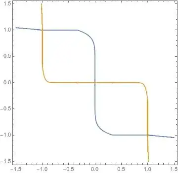
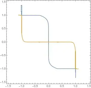
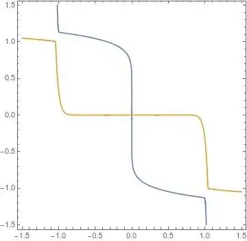
By performing the contour plot for some truncated approximations, we can infer for which the NR algorithm will work.

$$ \cases{ x + \frac{y^9}{3}+\frac{x^{243}}{9}=0 \\ y + \frac{x^{27}}{3}+\frac{y^{243}}{9}=0 \\ } $$

Here NR works with one solution.

$$ \cases{ x + \frac{y^9}{3}+\frac{x^{243}}{9} + \frac{y^{2187}}{27}=0 \\ y + \frac{x^{27}}{3}+\frac{y^{243}}{9} + \frac{x^{6561}}{27}=0 \\ } $$

Here NR succeeds with three solutions

$$ \cases{ x + \frac{y^9}{3}+\frac{x^{243}}{9} + \frac{y^{2187}}{27}+\frac{x^{59049}}{81}=0 \\ y + \frac{x^{27}}{3}+\frac{y^{243}}{9} + \frac{x^{6561}}{27}+\frac{y^{59049}}{81}=0 \\ } $$

Here NR only gives one solution. The two contours only cross one time.

In blue $f(x,y) = 0$ and in orange $g(x,y) = 0$