Expectation of $\Delta x$ and $\Delta y$
Since $\epsilon_d$ and $\epsilon_\alpha$ are independent random variables, and since $d, \theta,$ and $\alpha$ are all fixed constants at any particular time step, we have
$\mathbb{E}\Big[\Delta x\Big]=\mathbb{E}\Big[(d+\epsilon_d)\cos(\theta+\alpha+\epsilon_\alpha)\Big]$
$=\mathbb{E}\Big[d+\epsilon_d\Big]\mathbb{E}\Big[\cos(\theta+\alpha+\epsilon_\alpha)\Big]$
$=\big(\mathbb{E}\Big[d\Big]+\mathbb{E}\Big[\epsilon_d\Big]\big)\mathbb{E}\Big[\cos(\theta+\alpha+\epsilon_\alpha)\Big]$
$=(d+0)\mathbb{E}\Big[\cos(\theta+\alpha+\epsilon_\alpha)\Big]$
$=d\mathbb{E}\Big[\cos(\theta+\alpha+\epsilon_\alpha)\Big]$
and by the sum of angles rule,
$=d\mathbb{E}\Big[\cos(\theta+\alpha)\cos(\epsilon_\alpha)-\sin(\theta+\alpha)\sin(\epsilon_\alpha)\Big]$
$=d\bigg(\cos(\theta+\alpha)\mathbb{E}\Big[\cos \epsilon_\alpha \Big]-\sin(\theta+\alpha)\mathbb{E}\Big[\sin \epsilon_\alpha \Big]\bigg)$
Now, we can derive $\mathbb{E}\big[\cos \epsilon_\alpha \big] = e^{ - \frac{1}{2} \sigma_\alpha^2 }$ and $\mathbb{E}\big[\sin \epsilon_\alpha \big] = 0$ straightforwardly using Euler's formula, which says $e^{iX} = \cos X + i \sin X$ where $i=\sqrt{-1}$. If $X$~$N(0,\sigma)$ and we take the expectation of the equation, the left hand side becomes the moment generating function of a normal random variable $\mathbb{E} \big [ e^{iX} \big ] = e^{ \frac{1}{2} i^2 \sigma^2 + i \mu} = e^{ \frac{1}{2} (-1) \sigma^2 + i (0)} = e^{ - \frac{1}{2} \sigma^2 }$, and the equation becomes
$e^{ - \frac{1}{2} \sigma^2 } = \mathbb{E} \big [ \cos X + i \sin X \big ] = \mathbb{E} \big [ \cos X \big ] + i \mathbb{E} \big [ \sin X \big ]$
implying that $\mathbb{E} \big [ \cos X \big ] = e^{ - \frac{1}{2} \sigma^2 }$ and $\mathbb{E} \big [ \sin X \big ] = 0$ because $e^{ - \frac{1}{2} \sigma^2 }$ is a real number with no imaginary counterpart. More generally, for some $X$~$N(\mu,\sigma)$ and real constant $a$, we have $\mathbb{E}[\cos(aX)] = \cos( a \mu) e^{-\frac{1}{2} a^2 \sigma^2}$ and $\mathbb{E}[\sin(aX)]=\sin( a\mu) e^{ -\frac{1}{2} a^2 \sigma^2 }$. Many thanks to Parastoo Q, Hossein K. Mousavi, Danica, and Clement C. for these insights, linked here, here and here. We continue with the proof as follows...
$=d\bigg( e^{- \frac{1}{2} \sigma_\alpha^2} \cos(\theta+\alpha) - 0 \sin(\theta+\alpha) \bigg)$
so in conclusion...
$\mathbb{E}\Big[\Delta x\Big]= e^{-\frac{1}{2} \sigma_\alpha^2} d \cos(\theta+\alpha)$
and by similar logic,
$\mathbb{E}\Big[\Delta y\Big]= e^{-\frac{1}{2} \sigma_\alpha^2} d \sin(\theta+\alpha)$
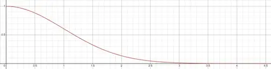
Note that as the variance in the steering angle decreases, i.e. $\sigma_\alpha^2 \to 0$, we have $e^{-\frac{1}{2} \sigma_\alpha^2} \to 1$ and $\Delta x \to d \cos (\alpha + \theta)$ and $\Delta y \to d \sin (\alpha + \theta)$ just as one would intuitively expect and just as every trig textbook would assert. However, as the variance in the steering angle increases, i.e. $\sigma_\alpha^2 \to \infty$, we have $e^{-\frac{1}{2} \sigma_\alpha^2} \to 0$ and $\Delta x \to 0$ and $\Delta y \to 0$, resulting in the drone experiencing no expected movement at all! This makes sense when we consider that, given a fixed distantce $d$, an increasingly unpredictable steering angle would cause the drone to move in the opposite $x$ and $y$ direction just as many times it would move in the intended $x$ and $y$ direction, resulting in no net change in location. So, every movement of the drone along the $x$ and $y$ axes is effectively weighted by the noise in the steering angle. The greater the noise, the smaller the weight and the less movement the drone is likely to experience; the smaller the noise, the greater the weight and the drone's movement is more likely to behave like a textbook trig formula. In a graph of $y=e^{-\frac{1}{2} \sigma_\alpha^2}$ below, we can observe how rapidly the weight approaches zero as a function of variance, reducing the intended movement of the drone by half with $\sigma_\alpha^2 \approx 1.2$
Variance of $\Delta x$ and $\Delta y$
I make use of a friendly formulation of variance as follows
$\mathbb{Var}[\Delta x] = \mathbb{Var}[(d+\epsilon_d)\cos(\theta+\alpha+\epsilon_\alpha)] $
$= \mathbb{E}\Big[\Big ((d+\epsilon_d)\cos(\theta+\alpha+\epsilon_\alpha) \Big )^2 \Big] - \mathbb{E}\Big[(d+\epsilon_d)\cos(\theta+\alpha+\epsilon_\alpha) \Big]^2$
by the proof above we have
$= \mathbb{E}\Big[(d+\epsilon_d)^2\cos^2(\theta+\alpha+\epsilon_\alpha) \Big] - \Big(
d \exp \left (-\frac{1}{2} \sigma_\alpha^2 \right ) \cos(\theta+\alpha) \Big)^2$
and once again because $\epsilon_d$ and $\epsilon_\alpha$ are independent,
$= \mathbb{E}\Big[(d+\epsilon_d)^2 \Big]\mathbb{E}\Big[\cos^2(\theta+\alpha+\epsilon_\alpha) \Big] - d^2 \exp \left (- \sigma_\alpha^2 \right ) \cos^2(\theta+\alpha)$
$= \mathbb{E}\Big[d^2 + 2d\epsilon_d + \epsilon_d^2 \Big]\mathbb{E}\Big[\cos^2(\theta+\alpha+\epsilon_\alpha) \Big] - d^2 \exp \left (- \sigma_\alpha^2 \right ) \cos^2(\theta+\alpha)$
$= \Bigg( d^2 + 2d\mathbb{E}\Big[\epsilon_d \Big] + \mathbb{E}\Big[\epsilon_d^2 \Big] \Bigg ) \mathbb{E}\Big[\cos^2(\theta+\alpha+\epsilon_\alpha) \Big] - d^2 \exp \left (- \sigma_\alpha^2 \right ) \cos^2(\theta+\alpha)$
We can derive $\mathbb{E}\Big[\epsilon_d^2 \Big]=\sigma_d^2$ via the moment generating function of the Gaussian distribution. Namely, given $X$~$N(\mu,\sigma)$, the $n$th moment of $X$ denoted as $E[X^2]$ is given by $\frac{d^n}{dt^n} M(t) |_{t=0}$ where $M(t)= \exp \Big ( \frac{\sigma^2 t^2}{2} + \mu t \Big )$. Hence,
$= \Bigg( d^2 + 2d(0)+ \sigma_d^2 \Bigg ) \mathbb{E}\Big[\cos^2(\theta+\alpha+\epsilon_\alpha) \Big] - d^2 \exp \left (- \sigma_\alpha^2 \right ) \cos^2(\theta+\alpha)$
$= \Bigg( d^2 + \sigma_d^2 \Bigg ) \mathbb{E}\Big[\cos^2(\theta+\alpha+\epsilon_\alpha) \Big] - d^2 \exp \left (- \sigma_\alpha^2 \right ) \cos^2(\theta+\alpha)$
We proceed by leveraging the power reduction rule
$= \Bigg( d^2 + \sigma_d^2 \Bigg ) \mathbb{E}\Big[ \frac{1}{2} \Big ( 1 + \cos2(\theta+\alpha+\epsilon_\alpha) \Big ) \Big] - d^2 \exp \left (- \sigma_\alpha^2 \right ) \cos^2(\theta+\alpha)$
$= \Bigg( d^2 + \sigma_d^2 \Bigg ) \frac{1}{2} \Bigg( 1 + \mathbb{E}\Big[ \cos \Big (2 (\theta+\alpha) + 2 \epsilon_\alpha \Big ) \Big] \Bigg) - d^2 \exp \left (- \sigma_\alpha^2 \right ) \cos^2(\theta+\alpha)$
again by the sum of angles rule
$= \Bigg( d^2 + \sigma_d^2 \Bigg ) \frac{1}{2} \Bigg( 1 + \mathbb{E}\Big[ \cos2(\theta+\alpha) \cos2 \epsilon_\alpha - \sin 2(\theta+\alpha) \sin 2\epsilon_\alpha \Big] \Bigg) - d^2 \exp \left (- \sigma_\alpha^2 \right ) \cos^2(\theta+\alpha)$
$= \Bigg( d^2 + \sigma_d^2 \Bigg ) \frac{1}{2} \Bigg( 1 + \cos2(\theta+\alpha) \mathbb{E}\Big[\cos2 \epsilon_\alpha \Big] - \sin 2(\theta+\alpha) \mathbb{E}\Big[ \sin 2\epsilon_\alpha \Big] \Bigg) - d^2 \exp \left (- \sigma_\alpha^2 \right ) \cos^2(\theta+\alpha)$
by the double angle rule for the sine function we have
$= \Bigg( d^2 + \sigma_d^2 \Bigg ) \frac{1}{2} \Bigg( 1 + \cos2(\theta+\alpha) \mathbb{E}\Big[\cos2 \epsilon_\alpha \Big] - 2 \mathbb{E}\Big[ \sin \epsilon_\alpha \cos \epsilon_\alpha \Big] \sin 2(\theta+\alpha) \Bigg) - d^2 \exp \left (- \sigma_\alpha^2 \right ) \cos^2(\theta+\alpha)$
In here I provide the derivation of $\mathbb{E}\Big[ \sin \epsilon_\alpha \cos \epsilon_\alpha \Big] = 0$. Thank you to heropup for offering some insight to get me on the right track.
$= \Bigg( d^2 + \sigma_d^2 \Bigg ) \frac{1}{2} \Bigg( 1 + \cos2(\theta+\alpha) \mathbb{E}\Big[\cos2 \epsilon_\alpha \Big] - 2 (0) \sin 2(\theta+\alpha) \Bigg) - d^2 \exp \left (- \sigma_\alpha^2 \right ) \cos^2(\theta+\alpha)$
$= \Bigg( d^2 + \sigma_d^2 \Bigg ) \frac{1}{2} \Bigg( 1 + \cos2(\theta+\alpha) \mathbb{E}\Big[\cos2 \epsilon_\alpha \Big] \Bigg) - d^2 \exp \left (- \sigma_\alpha^2 \right ) \cos^2(\theta+\alpha)$
by the double angle rule for the cosine function we have
$= \Bigg( d^2 + \sigma_d^2 \Bigg ) \frac{1}{2} \Bigg( 1 + \mathbb{E}\Big[2 \cos^2 \epsilon_\alpha - 1 \Big] \cos2(\theta+\alpha) \Bigg) - d^2 \exp \left (- \sigma_\alpha^2 \right ) \cos^2(\theta+\alpha)$
$= \Bigg( d^2 + \sigma_d^2 \Bigg ) \frac{1}{2} \Bigg( 1 + \Big ( 2 \mathbb{E}\Big[\cos^2 \epsilon_\alpha \Big] -1 \Big ) \cos2(\theta+\alpha) \Bigg) - d^2 \exp \left (- \sigma_\alpha^2 \right ) \cos^2(\theta+\alpha)$
Again, thank you to Danica for the following derivation linked here. Namely, for some $X$~$N(\mu,\sigma)$, we have $\mathbb{E}[\cos^2 X]= \frac{1}{2} ( 1 + e^{-2\sigma^2} \cos2\mu ) $ and $\mathbb{E}[\sin^2 X]= \frac{1}{2} ( 1 - e^{-2\sigma^2} \cos2\mu ) $. Hence, $\mathbb{E}[\cos^2 \epsilon_\alpha]= \frac{1}{2} ( 1 + e^{-2\sigma_\alpha^2} \cos 0 ) = \frac{1}{2} ( 1 + e^{-2\sigma_\alpha^2})$ and we continue with...
$= \Bigg( d^2 + \sigma_d^2 \Bigg ) \frac{1}{2} \Bigg( 1 + \Big ( 2 \cdot \frac{1}{2} (1 + e^{-2\sigma_\alpha^2}) -1 \Big ) \cos2(\theta+\alpha) \Bigg) - d^2 \exp \left (- \sigma_\alpha^2 \right ) \cos^2(\theta+\alpha)$
so in conclusion...
$\mathbb{Var}\Big[ \Delta x \Big] = \frac{1}{2} \Bigg( d^2 + \sigma_d^2 \Bigg ) \Bigg( 1 + e^{-2\sigma_\alpha^2} \cos2(\theta+\alpha) \Bigg) - e^{-\sigma_\alpha^2} d^2 \cos^2(\theta+\alpha)$
By similar logic,
$\mathbb{Var}\Big[ \Delta y \Big]= \frac{1}{2} \Bigg( d^2 + \sigma_d^2 \Bigg ) \Bigg( 1 - e^{-2\sigma_\alpha^2} \cos2(\theta+\alpha) \Bigg) - e^{-\sigma_\alpha^2} d^2 \sin^2(\theta+\alpha)$
What I find intriguing is that the variance in $\Delta y$ and $\Delta x$ is not only mediated by the noise in the steering angle $\sigma_\alpha^2$ and the noise in the distance $\sigma_d^2$ but also the steering angle $\alpha$ itself, the starting orientation $\theta$ itself, and the distance $d$ the drone intends to travel. This makes sense when you consider that, as we turn through some angle, the terminal end of a ray travels through a greater distance as the length of the ray grows. Similarly, given a ray of fixed length, the $\Delta x$ of the terminal end of the ray is greater in the area around a turn of $\frac{\pi}{2}$ rad than it is in the area around a turn of $\pi$ rad, while the $\Delta y$ of the terminal end of the ray is greater in the area around a turn of $\pi$ rad than it is in the area around a turn of $\frac{\pi}{2}$ rad.
In summary, let the angle $\theta$ and the ordered pair $(x,y)$ be the orientation and location of a drone in the plane at time $t$. Assuming the drone first turns in place by an angle $\alpha$ with Gaussian error $\epsilon_\alpha$~$N(0,\sigma_\alpha^2)$ and then moves forward by some distance $d$ with Gaussian error $\epsilon_d$~$N(0,\sigma_d^2)$, the expected location $(x',y')$ of the drone at time $t+1$ will be
$x' = x + \mathbb{E} \big [ \Delta x \big ] = x + e^{-\frac{1}{2} \sigma_\alpha^2} d \cos(\theta+\alpha)$
$y' = y + \mathbb{E} \big [ \Delta y \big ] = y + e^{-\frac{1}{2} \sigma_\alpha^2} d \sin(\theta+\alpha)$
Moreover, the variance in the change in $x$ and $y$ position, which could be used to weight a particular movement, is given by
$\mathbb{Var}\big[ \Delta x \big] = \frac{1}{2} \Big( d^2 + \sigma_d^2 \Big ) \Big( 1 + e^{-2\sigma_\alpha^2} \cos2(\theta+\alpha) \Big) - e^{-\sigma_\alpha^2} d^2 \cos^2(\theta+\alpha)$
$\mathbb{Var}\big[ \Delta y \big]= \frac{1}{2} \Big( d^2 + \sigma_d^2 \Big ) \Big( 1 - e^{-2\sigma_\alpha^2} \cos2(\theta+\alpha) \Big) - e^{-\sigma_\alpha^2} d^2 \sin^2(\theta+\alpha)$

