Model Predrictive Control is often used with Quadratic Programming. But I have tried Model Predictive Control with Linear Programming and it works very well.
Let's begin with the discrete SISO state space model:
$$x(k+1) = A_ax(k) + B_au(k)$$ $$y(k) = C_ax(k)$$
We apply integral action: $$A = \begin{bmatrix} A_a & B_a \\ 0 & I \end{bmatrix}$$
$$ B = \begin{bmatrix} 0 \\ I \end{bmatrix} $$
$$ C = \begin{bmatrix} C_a & 0 \end{bmatrix} $$
Then we create our extended model with controllability matrix $\Phi$ and our lower triangular toeplitz matrix that are a combination of observabillity matrix and controllability matrix.
$$\Phi = \begin{bmatrix} CA\\ CA^2\\ CA^3\\ \vdots \\ CA^{n-1} \end{bmatrix}$$
$$\Gamma = \begin{bmatrix} CB & 0 & 0 & 0 &0 \\ CAB & CB & 0 & 0 &0 \\ CA^2B & CAB & CB & 0 & 0\\ \vdots & \vdots &\vdots & \ddots & 0 \\ CA^{n-2} B& CA^{n-3} B & CA^{n-4} B & \dots & CA^{n-j} B \end{bmatrix}$$
Where $j=n$
Our goal is to solve x where $R$ is the reference vector and $U$ is the input signals and $x$ is the state vector.
$$R = \Phi x + \Gamma U$$
For finding the state vector $x$ we can use linear programming for this MPC problem.
$$Max: c^Tx$$ $$S.t: \tilde Ax \leq b$$ $$x \geq 0$$
Our linear programming model with $\lambda$ as the regularization parameter
$$\lambda = aI$$
$$c = (\Gamma^T \Gamma + \lambda)^T(R - \Phi x)$$
$$b = \Gamma^T (R - \Phi x)$$
$$\tilde A = \Gamma^T \Gamma + \lambda$$
You can see that I'm solving the tikhonov regularization problem with linear programming:
$$ x = (A^TA + aI)^{-1}A^Tb$$
Anyway!
I have used MataveControl library with LMPC function:
%% Parameters
A = [-0.313 56.7 0; -0.0139 -0.426 0; 0 56.7 0];
B = [0.232; 0.0203; 0];
C = [0 0 1];
D = [0];
delay = 0;
%% Model
aircraft = ss(delay, A, B, C, D);
%% Conver to discrete
h = 0.2;
sysd = c2d(aircraft, h);
%% Linear Model Predictive Control
Np = 20; % Number prediction
r = 20; % Reference value
T = 50; % Time limit
a = 0.5; % Regularization
I = 0.2; % Integral action (max = 0, min = 1)
%% Simulation
[y, t, x, u] = lmpc(sysd, Np, r, T, a, I);
%% Show the input signals
figure
plot(t, u)
title('Input signal')
grid on
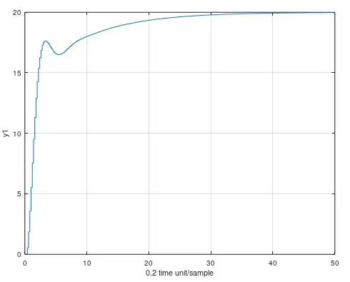
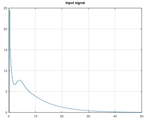
And the result was this. The MPC controller has built in integral action were the user can tune in the I parameter between 0 and 1. 0 for maximum integration and 1 for minimum integration. It's quite easy because the LMPC function only use the difference between new input signals with old input signals and use that as the input signals as the actual input signal for the model. Once the error is 0, then the difference between new and old input signals will also be 0.
Question:
If Linear programming works very well with MPC. Why are Quadratic Programming considered to be used?

