I will illustrate with with some geological data, known to have interesting autocorrelation. In the summer of 1987 rangers at Yellowstone National Park
measured times between eruptions of Old Faithful Geyser. This geyser is
well-known for its relatively regular eruptions, but it is not a clock. One
goal in collecting these data was to find a way to predict the time of the
next eruption for the convenience of tourists waiting to see an eruption.
Data (in minutes) for $n = 107$ (almost) consecutive waiting times are as follows:
x = c(78, 74, 68, 76, 80, 84, 50, 93, 55, 76, 58, 74, 75, 80, 56, 80, 69, 57,
      90, 42, 91, 51, 79, 53, 82, 51, 76, 82, 84, 53, 86, 51, 85, 45, 88, 51,
      80, 49, 82, 75, 73, 67, 68, 86, 72, 75, 75, 66, 84, 70, 79, 60, 86, 71,
      67, 81, 76, 83, 76, 55, 73, 56, 83, 57, 71, 72, 77, 55, 75, 73, 70, 83,
      50, 95, 51, 82, 54, 83, 51, 80, 78, 81, 53, 89, 44, 78, 61, 73, 75, 73,
      76, 55, 86, 48, 77, 73, 70, 88, 75, 83, 61, 78, 61, 81, 51, 80, 79)
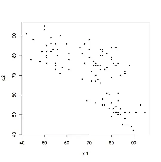
In order to see if the wait for the last eruption is useful in predicting the wait for the next, one can consider the correlation between the vector
$x_1 = (78, 74, 68, \dots, 51, 80)$ and the vector $x_2 = (74, 68, \dots, 80, 79),$ which is 'lagged' by one eruption.
The correlation is $r_{1,2} = -0.685,$ indicating that short waits tend to be followed by long ones. as shown in the plot below. The calculation of the autocorrelation in R statistical software is:
x.1 = x[1:106];  x.2 = x[2:107];  cor(x.1, x.2)
## -0.6849171
The autocorrelation function (ACF) shows correlations for several lags (of order
2, 3, 4, etc.) in addition to the lag of order 1 just illustrated.
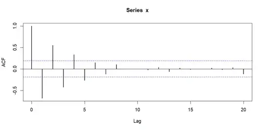
The first few lags show alternate negative and positive autocorrelations.
Autocorrelations that fall within the band marked by the dotted blue lines are deemed not to be significantly different from $0.$ (Of course, the autocorrelation for 'lag 0' is just the correlation $r = 1$ of $x$ with itself.)
While it is impossible to say whether a time series (economic or geological) will continue past behavior into the future, autocorrelation methods have
proved effective in some kinds of short-range forecasting.
In the Old Faithful example, the length of the wait for the last eruption did provide a useful guide to predicting the wait for the next eruption. In fact,
these inter-eruption times form a Markov Chain in which several past eruptions
still provide useful predictive information (until the 'one-step' dependence
of the Markov chain 'wears off'.)
Notes: (1) The usual definition of correlation
$$r_{xy} = \frac{\sum_{i=1}^n (X_i - \bar X)(Y_i - \bar Y)}{S_XS_y},$$
where $\bar X$ and $\bar Y$ are sample means and $S_X$ and $S_Y$ are
sample standard deviations, is somewhat modified for autocorrelations
because $X$ and $Y$ are the same, except for the lag. The modifications are
that the sample means and SDs for the whole series are used, and the sum is
taken over $n - \ell$ terms, where $\ell$ is the order of the lag.
(2) I said that the eruptions in the series $x$ are 'almost' consecutive.
In fact, there are a few gaps where nighttime eruptions are missing, but
they do not interfere with the fundamental story about autocorrelation.
(3) Since these data were collected, there have been several earthquakes near Old Faithful geyser, which have rearranged the underground 'plumbing' for
hot water feeding the geyser. So recent data on inter-eruption times are
slightly different. Several websites undertake to provide contemporaneous data.
(4) You may find the Wikipedia article on autocorrelation useful. (But the notation is not the same as I am used to.)

