4

Consider the system $$\begin{aligned} \dot{x} &=-y-x^3+x^3y^2\\ \dot{y}&=x-y^3+x^2y^3\end{aligned}$$ Show that the equilibrium point $(0,0)$ is asymptotically stable and an estimate of its attractiveness basin.


Clearly the point $(0,0)$ is a point of equilibrium and also $D_f(x,y)=\begin{pmatrix}-3x^2+3y^4 & -1+2yx^3\\ 1+2xy^3 &-3y^2+3y^2x^2 \end{pmatrix}$, so $D_f(0,0)=\begin{pmatrix}0 & -1\\1 &0 \end{pmatrix}$ and has eigenvalues ​​$ \pm i$ So, I can not conclude anything of stability for this point, I need a Liapunov function and I do not know what it is or how to find it, could someone help me please? Thank you very much.

user402543
  • 1,183
  • 3
    Always try the simplest one first. For example, quadratic. More precisely, $V(x, y) = x^2+y^2$. – Evgeny Oct 30 '17 at 05:44

3 Answers3

4

In addition to what has been said by @Evgeny and @MrYouMath: the set $$ M=\left\{ (x,y)\in\mathbb R^2 :\; x^2+y^2<2 \right\} $$ is a positively invariant set of the considered system since $\forall (x,y)\in M$ $$ \dot V=-x^4-y^4+x^2y^2(x^2+y^2)<-x^4-y^4+2x^2y^2=-(x^2-y^2)^2\leq 0; $$ it is also a subset (guaranteed estimation) of the domain of attraction.

AVK
  • 5,333
3

As @Evgeny suggested you could use the Lyapunov function candidate

$$V(x,y)=\dfrac{1}{2}\left[x^2+y^2\right].$$

$V(x,y)$ is clearly positive definite at the origin and radially unbounded (which we would need for assessing global asymptotic stability).

The time derivative of $V(x,y)$ is given by $$\dot{V}=x\dot{x}+y\dot{y}=x(-y-x^3+x^3y^2)+y(x-y^3+x^2y^3)$$ $$\dot{V}=-x^4-y^4+x^2y^2(x^2+y^2)=-(1-y^2)x^4-(1-x^2)y^4.$$

As the lower order terms $-x^4-y^4$ are negative definite we can conclude that the equilibrium point is asymptotically stable in a region around the origin. Using the comment given by @Evgeny we can see that this expression is negative semidefinite if $(x,y)$ lie inside the unit circle $D=\{(x,y)\in \mathbb{R}^2|x^2+y^2<1\}$. This is the basin of attraction (correction due to @Artem).

We cannot say if the origin is globally asymptotically stable because $\dot{V}$ is not negative definite for all regions around the origin. This does not mean that the origin cannot be globally asymptotically stable. It just means we can only show (local) asymptotic stability of the origin with $V(x)$ as our Lyapunov function candidate.

MrYouMath
  • 16,174
  • 3
    Actually, you can do better if regroup terms correctly: $\dot{V} = -x^4(1-y^2)-y^4(1-x^2)$. This also gives a rough estimate of basin of attraction since this expression is negative when $\vert x \vert < 1$ and $\vert y \vert < 1$. – Evgeny Oct 30 '17 at 13:18
  • 1
    @Evgeny: You are right. I felt that I should be able to factor this expression. – MrYouMath Oct 30 '17 at 13:19
  • 1
    Also, speaking about radial unboundedness: it's not a necessary condition really, see recent discussion in comments. – Evgeny Oct 30 '17 at 18:09
  • 1
    It is not necessary for asymptotic stability but it is necessary for global asymptotic stability (see the comment in the brackets in my answer). I think that is what the example showed. Or do you mean something else? – MrYouMath Oct 30 '17 at 18:14
  • 1
    Even for the global asymptotic stability it is not necessary. You can prove the global asymptotic stability with a Lyapunov function which is not radially unbounded. Moreover, you can transform the image of any Lyapunov function such that it will become bounded but still will prove that something is globally asymptotic stable. – Evgeny Oct 30 '17 at 20:29
  • 1
    Really? Why do many textbooks assume radial inboundedness? Can you give reference to that? – MrYouMath Oct 30 '17 at 20:35
  • I've already linked the discussion in the comments to another question. I don't really know why this condition is so omnipresent. Maybe this is the easiest condition. – Evgeny Oct 31 '17 at 05:28
  • 1
    The conclusion about the basin of attraction is incorrect. – Artem Oct 31 '17 at 18:20
  • @Artem: Could you elaborate on that? – MrYouMath Oct 31 '17 at 19:35
  • The negative sign of the derivative of the Lyapunov function does not mean the point is in the basin of attraction. You need to look at the sets ${x\colon V(x)\leq \alpha}$, which in your case are discs. – Artem Oct 31 '17 at 22:00
  • @Artem Sorry for my late edit, but yesterday I had a lot of work to do. And I also had to think about your comment. Thank you, I learned something new today :). – MrYouMath Nov 02 '17 at 06:58
0

This problem can be handled with an optimization procedure, having in mind that generally is a non convex problem. The result depends on the test Lyapunov function used so we will generalize to a quadratic Lyapunov function

$$ V(p) = p^{\dagger}\cdot M\cdot p = a x^2+b x y + c y^2,\ \ \ p = (x,y)^{\dagger} $$

and

$$ f(p) = \{-y - x^3 + x^3 y^2, x - y^3 + x^2 y^3\} $$ with $a>0,c>0, a b-b^2 > 0$ to assure positivity on $M$. We will assure a set involving the origin $Q_{\dot V}$ such that $\dot V(Q_{\dot V}) < 0$. The optimization process will be used to guarantee a maximal $Q_{\dot V}$.

After determination of $\dot V = 2 p^{\dagger}\cdot M\cdot f(p)$ we follow with a change of variables

$$ \cases{ x = r\cos\theta\\ y = r\sin\theta } $$

so $\dot V = \dot V(a,b,c,r,\theta)$. The next step is to make a sweep on $\theta$ calculating

$$ S(a,b,c, r)=\{\dot V(a,b,c,r,k\Delta\theta\},\ \ k = 0,\cdots, \frac{2\pi}{\Delta\theta} $$

and then the optimization formulation follows as

$$ \max_{a,b,c,r}r\ \ \ \ \text{s. t.}\ \ \ \ a > 0, c> 0, a c -b^2 > 0, \max S(a,b,c,r) \le -\gamma $$

with $\gamma > 0$ a margin control number.

Follows a MATHEMATICA script which implements this procedure in the present case.

f = {-y - x^3 + x^3 y^2, x - y^3 + x^2 y^3};
V = a x^2 + 2 b x y + c y^2;
dV = Grad[V, {x, y}].f /. {x -> r Cos[t], y -> r Sin[t]};
rest = Max[Table[dV, {t, -Pi, Pi, Pi/30}]] < -0.1;
rests = Join[{rest}, {r > 0, a > 0, c > 0, a c - b^2 > 0}];
sols = NMinimize[Join[{-r}, rests], {a, b, c, r}, Method -> "DifferentialEvolution"]
rest /. sols[[2]]

dV0 = Grad[V, p].f /. sols[[2]] V0 = V /. sols[[2]] r0 = 2; rmax = r /. sols[[2]]; gr0 = StreamPlot[f, {x, -r0, r0}, {y, -r0, r0}]; gr1a = ContourPlot[dV0, {x, -r0, r0}, {y, -r0, r0}, ContourShading -> None, Contours -> 80]; gr1b = ContourPlot[dV0 == 0, {x, -r0, r0}, {y, -r0, r0}, ContourStyle -> Blue]; gr2 = ContourPlot[x^2 + y^2 == rmax^2, {x, -r0, r0}, {y, -r0, r0}, ContourStyle -> {Red, Dashed}]; Show[gr0, gr1a, gr1b, gr2]

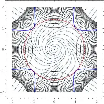
Follows a plot showing in black the level sets $Q_{\dot V}$ an in blue the trace of $\dot V = 0$. In dashed red is shown the largest circular set $\delta = 1.42486$ defining the maximum attraction basin for the given test Lyapunov function's family.

enter image description here

Cesareo
  • 36,341