What is the implication of Perron Frobenius Theorem?

Question

The Perron Frobenius theorem states:

Any square matrix $A$ with positive entries has a unique eigenvector with positive entries (up to a multiplication by a positive scalar), and the corresponding eigenvalue has multiplicity one and is strictly greater than the absolute value of any other eigenvalue.

---

So I tempted fate using this matrix:

$$ A =\begin{bmatrix} 1 & 1 \\ 1 & 1 \end{bmatrix}$$

I find my eigenvalues to be $\lambda_1 = 0, \lambda_2 = 2$

Now I find my eigenvector, taking $v_{11} = 1$, $v_{21} = 1$

I find $v_1 = \begin{bmatrix} v_{11} & v_{12} \end{bmatrix}$ = $\begin{bmatrix} 1 & -1 \end{bmatrix}$

$v_1 = \begin{bmatrix} v_{21} & v_{22} \end{bmatrix}$ = $\begin{bmatrix} 1 & 1 \end{bmatrix}$

This verifies the Perron-Frobenius theorem.

---

Now what is the great implication that every positive square matrix has a real eigenvector with an eigenvalue that is the largest of all eigenvalues?

Can someone show me an application of this theorem?

Answer 1

The Perron-Frobenius theorem is used in Google's Pagerank. It's one of the things that make sure that the algorithm works. Here it's explained why the the theorem is useful, you have a lot of information with easy explanations on Google.

Answer 2

For example, there are important applications in the theory of finite Markov chains. Among other things, it implies that a Markov chain with strictly positive transition probabilities has a unique stationary distribution.

Answer 3

First of all, the conclusion is more interesting if you also try an example where the matrix entries are still real, but not positive. For example, if $A$ is the $2\times2$ rotation matrix $$A=\pmatrix{\cos\theta&\sin\theta\\ -\sin\theta&\cos\theta}$$ then you can check that the eigenvectors are no longer real, and there's no longer a unique eigenvalue of maximum modulus: the two eigenvalues are $e^{i\theta}$ and $e^{-i\theta}$.

I second Robert Israel's nomination of Markov chains as a great application. I'll add the following, though. (I'll remark that you don't actually need the matrix to have positive entries - just for some power of it to have positive entries.) Suppose you have a finite connected graph (or strongly connected digraph) such that the gcd of the cycle lengths is $1$. Then if $A$ is the adjacency matrix for the graph, some power $A^r$ will have positive entries so Perron-Frobenius applies. Since the entries of $A^n$ count paths in the graph, we conclude that for any pair of vertices in the graph, the number of paths of length $n$ between them is $c\lambda_1^n(1+o(1))$, where $\lambda_1$ is the Perron-Frobenius eigenvalue and $c$ is a computable constant. Applications of this particular consequence of Perron-Frobenius include asymptotic growth rate results for "regular languages," which are defined in terms of paths on graphs.

In particular, there is a cute formula giving the $n$-th Fibonacci number as $$F_n=\left\langle \frac1{\sqrt5}\phi^n\right\rangle$$ where $\phi$ is the "golden ratio" $(1+\sqrt5)/2$ and $\langle\cdot\rangle$ denotes "closest integer." This formula, and many others like it, become less surprising once you check that $$\pmatrix{1&1\\1&0}^n=\pmatrix{F_{n+1}&F_n\\ F_n&F_{n-1}}$$ and note that $\phi$ is the Perron-Frobenius eigenvalue (and the other eigenvalue is smaller than $1$ in absolute value.)

Answer 4

I would like to add an engineering application. I am a researcher from a wireless communication background. One of the most fundamental problem in our area would be the so-called Power Control wherein a mobile tower transmitting individual data to the several mobiles has to minimize its own power consumption meanwhile ensuring a minimum level of signal quality at the mobile. This can be formalized as a non-convex optimization problem. However, using some theoretical tools based on the perron-frobenius theory, you can find a simple, iterative algorithm which finds the true solution to this problem. This result has been a break through in our field. The perron-frobenius eigenvector will be the sort of numbers (positive) which states how much power the mobile tower has to use to serve its users. A well-cited paper in this regard is "A framework for uplink power control in cellular radio systems", in case you are interested to read more about this.

Answer 5

One of the nice things about it is that for $v$ a vector with all positive entries, if we let $v_k = A^k v$, then $\lim_{k\to\infty} \frac{v^k}{|| v_k ||}$ exists and is an eigen vector for the Perron-Frobenius eigen value.

Answer 6

I'll add an answer from the world of symbolic dynamics and tiling theory.

If you have a substitution on some alphabet $\mathcal{A}=\{a_1,\ldots,a_k\}$, say something like the Fibonacci substitution $$\sigma\colon\begin{cases}a\mapsto ab\\ b\mapsto a\end{cases}$$ then you have an associated transition matrix $M_{\sigma}$ where $m_{ij}$ is the number of times the letter $a_i$ appears in the word $\sigma(a_j)$. So for example the transition matrix for the Fibonacci substitution is $M_{\sigma}=\left(\begin{smallmatrix}1&1\\ 1&0\end{smallmatrix}\right)$.

Whenever there exists a $k$ such that $M_{\sigma}^k$ has strictly positive entries, we say that $\sigma$ is a primitive substitution. Transition matrices of primitive substitutions therefore satisfy the hypothesis of the Perron Frobenius theorem and we can say the following thanks to it.

Theorem Let $|w|$ be the length of a word. If $\sigma$ is a primitive substitution, then the PF eigenvalue $\lambda_{PF}$ has the property that $\lim_{n\to \infty} |\sigma^n(a_i)|/\lambda_{PF} = 1$ for any $a_i\in\mathcal{A}$. That is, the length of the words $\sigma^n(a_i)$ are roughly $\lambda_{PF}^n$.

If $v_{PF}$ is the associated dominant right eigenvector then the frequency of letters in the limit word $\sigma^{\infty}(a_j)$ is given by $\mbox{freq}(a_i)=(v_{PF})_i/\|v_{PF}\|_1$, and this is independent of choice of seed letter $a_j$.

We can use the left eigenvector to assign lengths to intervals in the line which are labelled by the symbols $a_i$, and we can then think of $\lambda_{PF}$ as being a natural expansion factor for a geometric substitution, whereby we apply $\sigma$ to the interval assigned the letter $a_i$ by expanding it by a factor of $\lambda_{PF}$ and then cutting it up into intervals of lengths associated to the eigenvector, and in the order prescribed by the substitution.

A good paper to read more about this stuff, including how we can similarly do substitutions in higher dimensions is this paper by Natalie Priebe-Frank.

Answer 7

To check the stability of dynamical systems, one can try to search for a real-valued positive function named Lyapunov function.

If the dynamical system is LTI, that is, of the format $$ \dot{x}(t) = Ax(t) $$ or $$ x(k+1) = Ax(k),$$ one can restrict the search for quadratic Lyapunov functions, that is, for functions $V: \mathbb{R}^n \rightarrow \mathbb{R}$ of the format $V(x) = x^T P x$.

If the LTI system is also positive (that is, the state is always guaranteed to be in the positive orthant of $\mathbb{R}^n$), it is possible to use Perron-Frobenius theorem to prove that this search can be restricted to linear functions, simplifying even more the problem of stability analysis. For details, see slides 31-37 of Prof. Boyd's lecture notes on Perron-Frobenius theory.

You can also check the following reference for an embracing survey of applications:

Pillai, S. Unnikrishna, Torsten Suel, and Seunghun Cha. "The Perron-Frobenius theorem: some of its applications." IEEE Signal Processing Magazine 22.2 (2005): 62-75.

Answer 8

Forecasting the Future with a Positive Stochastic Matrix

My favorite application is: forecast the future!

I will give an example I use in presentations to undergrads. Some words in the images are in portuguese but you do not need to understand that.

Imagine three buckets that initially contain a total of $1$ Kg of sand:

At every step, sand is redistributed according to fixed percentages in the image below. I move 20% of the sand of the bucket $V$ to the bucket $A$, 50% of the sand in the bucket $V$ to the bucket $L$,...

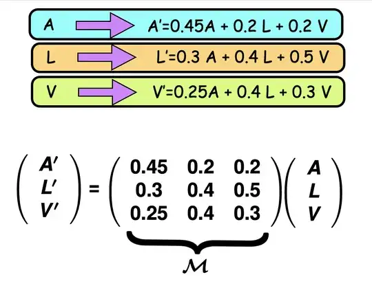
Let the starting distribution be $(A,L,V)$ and the distribution after one step be $(A',L',V')$.
Because the rule is linear we have $$ (A',L',V') \;=\; M\,(A,L,V), $$ where $M$ is a matrix that has two notable properties:

(1) All entries are positive. One application of the process mixes the sand thoroughly—some sand from every bucket ends up in every other bucket.

(2) Each column sums to 1. No sand is lost or added during the transfer.

Such a matrix is called a positive stochastic matrix.

Now repeat the same procedure indefinitely. The natural question is:

What happens to the sand distribution after many iterations?

This is kind of complicate, since to calculate the distribution of the sand after $n$ iterations you would need to calculate $M^n$ and multiply by the original distribution $(A,L,V)$

which is tedious by hand. Since computer can do this very fast, we can do an experiment using a spreadsheet software. It is quite easy. You see below two of my experiments

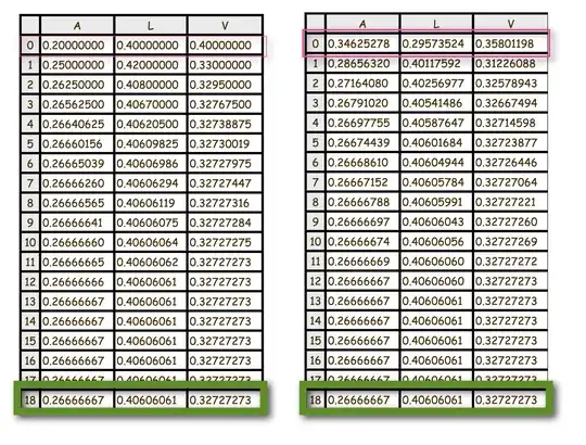
in the first experiment I put 0.200 Kg in bucket A 0.400 Kg in bucket L 0.400 Kg in bucket V

and I repeat the process 18 times. In the end I got the distribution

(0.2666667, 0.40606061, 0.32727273)

Surprisingly, the distribution of sand stabilises after only four iterations—already matching to three decimal places!

Even more remarkable is that, if I begin with a completely different initial distribution, the sand still settles into the same stable pattern. In the second experiment I chose random amounts for the first two buckets, then added enough sand to the third so the total mass was exactly 1 kg. Once again, the distribution converged to the same limit. Try as many distinct 1 kg distributions as you like—the outcome is always identical!

What is this special distribution (0.2666667, 0.40606061, 0.32727273)? Well this is (approximately ) the distribution

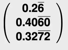
and this vector is an eigenvector for the eigenvalue $1$! Indeed $1$ is the eigenvalue with the largest modulus of the matrix $M$ and its eigen-space is generated by this positive vector. This vetor is the only $1$-eigenvector whose sum of coordinates is $1$.

Like I said, this lets you forecast the future sand distribution in this linear system: even if you don’t know the starting layout (only the total amount of sand), after a few rounds the mix will be very, very close to that 1-eigenvector. Just run the experiment once and you’ve got the answer!

The Perron--Frobenius Theorem says this trick scales to any number of buckets. Got $10^{23}$ of them? As long as your mixing matrix is positive (every entry $>0$) and you’re not losing or adding sand, it doesn’t matter how you first spread the 1kg. Keep repeating the mix and, as $n \to \infty$, the sand always settles into one special vector---the unique eigenvector for eigenvalue $1$ whose coordinates add up to $1$. You can even estimate the rate of convergence (that is always exponential).

MAGIC!

There’s a similar idea for continuous mass distributions driven by chaotic dynamical systems. In that setting, the mass evolution is modeled by a positive linear operator acting on a space of functions (or distributions). This operator—known as the transfer operator (or Ruelle–Perron–Frobenius operator)—is a cornerstone of Ergodic Theory for analyzing the dynamics of (piecewise) smooth maps.