I inspired by this notebook, and I'm experimenting IsolationForest algorithm using scikit-learn==0.22.2.post1 for anomaly detection context on the SF version of KDDCUP99 dataset, including 4 attributes. The data is directly fetched from sklearn and after preprocessing (label encoding the categorical feature) passed to the IF algorithm with the default setup.
The full code is as follows:
from sklearn import datasets
from sklearn import preprocessing
from sklearn.model_selection import train_test_split
from sklearn.ensemble import IsolationForest
from sklearn.metrics import confusion_matrix
from sklearn.metrics import recall_score, roc_curve, roc_auc_score, f1_score, precision_recall_curve, auc
from sklearn.metrics import make_scorer
from sklearn.metrics import accuracy_score
import pandas as pd
import numpy as np
import seaborn as sns
import itertools
import matplotlib.pyplot as plt
import datetime
%matplotlib inline
def byte_decoder(val):
# decodes byte literals to strings
return val.decode('utf-8')
#Load Dataset KDDCUP99 from sklearn
target = 'target'
sf = datasets.fetch_kddcup99(subset='SF', percent10=True) # you can use percent10=True for convenience sake
dfSF=pd.DataFrame(sf.data,
columns=["duration", "service", "src_bytes", "dst_bytes"])
assert len(dfSF)>0, "SF dataset no loaded."
dfSF[target]=sf.target
anomaly_rateSF = 1.0 - len(dfSF.loc[dfSF[target]==b'normal.'])/len(dfSF)
"SF Anomaly Rate is:"+"{:.1%}".format(anomaly_rateSF)
#'SF Anomaly Rate is: 0.45%'
#Data Processing
toDecodeSF = ['service']
apply hot encoding to fields of type string
convert all abnormal target types to a single anomaly class
dfSF['binary_target'] = [1 if x==b'normal.' else -1 for x in dfSF[target]]
leSF = preprocessing.LabelEncoder()
for f in toDecodeSF:
dfSF[f + " (encoded)"] = list(map(byte_decoder, dfSF[f]))
dfSF[f + " (encoded)"] = leSF.fit_transform(dfSF[f])
for f in toDecodeSF:
dfSF.drop(f, axis=1, inplace=True)
dfSF.drop(target, axis=1, inplace=True)
#check rate of Anomaly for setting contamination parameter in IF
dfSF["binary_target"].value_counts() / np.sum(dfSF["binary_target"].value_counts())
#data split
X_train_sf, X_test_sf, y_train_sf, y_test_sf = train_test_split(dfSF.drop('binary_target', axis=1),
dfSF['binary_target'],
test_size=0.33,
random_state=11,
stratify=dfSF['binary_target'])
#print(y_test_sf.value_counts())
#1 230899
#-1 1114
#Name: binary_target, dtype: int64
#y_test_sf.value_counts() / np.sum(y_test_sf.value_counts())
1 0.954984
#-1 0.045016
#Name: binary_target, dtype: float64
#GridSearch IF parameters (SF)
scoring = {'AUC': 'roc_auc', 'Recall': make_scorer(recall_score, #f1_score
pos_label=-1)}
gs_cont_sf = GridSearchCV(IsolationForest(n_jobs=-1),
param_grid={'n_estimators': [2], #[2**i for i in range(1, 9)],
'max_samples': np.arange(0.1, 1.0, 0.2),
'contamination': [0.001, 0.003, 0.005, 0.01, 0.1, 0.2, 0.3]
},
scoring=scoring, refit='Recall', return_train_score=True, cv=3, verbose=1, n_jobs=-1)
gs_cont_sf.fit(X_train_sf, y_train_sf)
results = gs_cont_sf.cv_results_
contamination, max_samples, n_estimators = tuple(pd.DataFrame(results).iloc[np.argmax(pd.DataFrame(results)["mean_test_Recall"])][["param_contamination", "param_max_samples", "param_n_estimators"]].to_numpy().tolist())
contamination, max_samples, n_estimators
##training IF Model - SF ver. and predict the outliers/anomalies on the test-set with final GridSearchCV results
iso_for_sf = IsolationForest(random_state=11,
n_estimators=n_estimators, #2
max_samples=max_samples, #0.1
contamination=contamination, #0.3 real is 0.045!
n_jobs=-1)
iso_for_sf.fit(X_train_sf, y_train_sf)
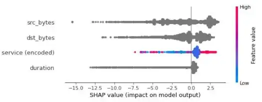
Create shap values and plot outliers summary_plot for test-set
X_explain = X_test_sf
shap_values = shap.TreeExplainer(iso_for_sf).shap_values(X_explain)
shap.summary_plot(shap_values, X_explain)
#plot 2
sampled_data = X_train_sf.sample(100)
shap.initjs()
explainer = shap.TreeExplainer(iso_for_sf)
shap_values = explainer.shap_values(sampled_data)
shap.force_plot(explainer.expected_value, shap_values, sampled_data)
- Why 3 features contributions are depicted with a grey color, which is out of the bar color range?
- What is the interpretation of the following
shap.summary_plotandshap.force_plotin terms of outliers? - Is it clear how the SHAP toolset could transparent the contribution of features concerning outliers/anomalies?
shap.summary_plot for all samples in test-set:
shap.force_plot for 100 samples in train-set:

Probably I am missing something here, and any help will be highly appreciated.