Gini impurity in decision tree (reasons to use it)

Question

In a decision tree, Gini Impurity[1] is a metric to estimate how much a node contains different classes. It measures the probability of the tree to be wrong by sampling a class randomly using a distribution from this node:

$$ I_g(p) = 1 - \sum_{i=1}^J p_i^2 $$

If we have 80% of class C1 and 20% of class C2, labelling randomly will then yields 1 - 0.8 x 0.8 - 0.2 x 0.2 = 0.32 Gini impurity value.

However, assigning randomly a class using the distribution seems like a bad strategy compared with simply assigning the most represented class in this node (in above example, you would just label C1 all the time and get only 20% of error instead of 32%).

In that case, I would be tempted to simply use this as a metric, since it is also the probability of mislabeling :

$$ I_m(p) = 1 - \max_i [ p_i] $$

Is there a deeper reason to use Gini and/or a good reason not to use this approach instead ? (In other words, Gini seems to over-estimate the mislabellings that will happen, isn't it ?)

[1] https://en.wikipedia.org/wiki/Decision_tree_learning#Gini_impurity

---

EDIT: Motivation

Suppose you have two classes $C_1$ and $C_2$, with probabilities $p_1$ and $p_2$ ($1 \ge p_1 \ge 0.5 \ge p_2 \ge 0$, $p_1 + p_2 = 1$).

You want to compare strategy "always label $C_1$" with strategy "label $C_1$ with $p_1$ probability, and $C_2$ with $p_2$ probability", thus the probability of success are respectively $p_1$ and $p_1^2 + p_2^2$.

We can rewrite this second one to:

$$ p_1^2 + p_2^2 = p_1^2 + 2p_1p_2 - 2p_1p_2 + p_2^2 = (p_1 + p_2)^2 - 2p_1p_2 = 1 - 2p_1p_2 $$

Thus, if we substract it to $p_1$:

$$ p_1 - 1 + 2p_1p_2 = 2p_1p_2 - p_2 = p_2 ( 2p_1 - 1) $$

Since $p_1 \ge 0.5$, then $p_2 ( 2p_1 - 1) \ge 0$, and thus:

$$ p_1 \ge p_1^2 + p_2^2 $$

So choosing the class with highest priority is always a better choice.

---

EDIT: Choosing an attribute

Suppose now we have $n_1$ items in $C_1$ and $n_2$ items in $C_2$. We have to choose which attribute $a \in A$ is the best to split the node. If we use superscript $n^v$ for number of items that have a value $v$ for a given attribute (and $n^v_1$ items of $C_1$ that have value $v$), I propose we use the score:

$$ \sum_v \frac{n^v}{n_1 + n_2} \frac{max(n^v_1, n^v_2)}{n^v_1 + n^v_2} $$

As a criterion instead of Gini.

Note, since $n^v = n^v_1 + n^v_2$ and $n_1 + n_2$ doesn't depend on the choosen attribute, this can be rewritten:

$$ \sum_v max(n^v_1, n^v_2) $$

And simply interpreted as the number of items in the dataset that will be properly classified.

Answer 1

I believe this issue is addressed in the Elements of Statistical Learning (https://hastie.su.domains/ElemStatLearn/printings/ESLII_print12_toc.pdf.download.html) around pg. 360 (maybe slightly different depending on the edition you have):

"We classify the observations in node $m$ to class $k(m) = \arg\max_k > \hat{p}_{mk}$, the majority class in node $m$. Different measures $Q_m(T)$ of node impurity include the following:

• Misclassification error: $1 - \hat{p}_{mk(m)} = \frac{1}{N_m} \sum_{i \in R_m} \mathbb{I}(y_i > \neq k(m)).$

• Gini index: $ \sum_{k \neq k'} \hat{p}_{mk} \hat{p}_{mk'} = \sum_{k=1}^K \hat{p}_{mk} (1 - \hat{p}_{mk}). $

• Cross-entropy or deviance: $ -\sum_{k=1}^K \hat{p}_{mk} \log \hat{p}_{mk}. $

For two classes, if $p$ is the proportion in the second class, these three measures are $1 - \max(p, 1 - p)$, $2p(1-p)$, and $-p\log p - > (1-p)\log(1-p)$, respectively. They are shown in Figure 9.3. All three are similar, but cross-entropy and the Gini index are differentiable, and hence more amenable to numerical optimization.

Comparing equations (9.13) and (9.15), we see that we need to weight the node impurity measures by the number $N_{mL}$ and $N_{mR}$ of observations in the two child nodes created by splitting node $m$.

In addition, cross-entropy and the Gini index are more sensitive to changes in the node probabilities than the misclassification rate. For example, in a two-class problem with 400 observations in each class (denoted by $(400, 400)$), suppose one split creates nodes $(300, > 100)$ and $(100, 300)$, while another split creates nodes $(200, 400)$ and $(200, 0)$. Both splits produce a misclassification rate of 0.25, but the second split produces a pure node and is probably preferable. Both the Gini index and cross-entropy are lower for the second split. For this reason, either the Gini index or cross-entropy should be used when growing the tree. To guide cost-complexity pruning, any of the three measures can be used, but typically it is the misclassification rate.

The Gini index can be interpreted in two interesting ways. Rather than classify observations to the majority class in the node, we could classify them to class $k$ with probability $\hat{p}_{mk}$. Then the training error rate of this rule in the node is $\sum_{k \neq k'} > \hat{p}_{mk} \hat{p}_{mk'}$—the Gini index. Similarly, if we code each observation as 1 for class $k$ and 0 otherwise, the variance over the node of this 0-1 response is $\hat{p}_{mk}(1 - \hat{p}_{mk})$. Summing over classes $k$ again gives the Gini index."

Answer 2

Misclassification error will not help in splitting the Tree.
Reason-We consider the weighted dip of error from parent Node to the child node and misclassification error will always result in 0(Other than pure splits).

Let's consider an example
Data = 1, 1, 0, 1, 0, 1, 0, 1, 0, 1
Parent Classification error= 4/10 = 0.4
Parent Gini Impurity = 1-(0.4x0.4+0.6x0.6) = 0.48

Case - I
Split - 1, 1, 0, 1 Vs 1, 0, 1, 0, 1, 0
Classification error= 0.4x0.25 + 0.6x0.5 = 0.4, split not possible
Gini Impurity = 0.45

Case - II
Split - 1, 1, 1, 0, 0 Vs 0, 1, 0, 1, 0
Classification error = 0.5x0.4 + 0.5x0.4 = 0.4, split not possible
Gini Impurity = 0.48

Case - III
Split - 1, 1, 0, 0, 1, 1 Vs 1, 0, 1, 0
Classification error = 0.6x(2/6) + 0.4x0.5 = 0.4, split not possible
Gini Impurity = 0.477

Pure splits
Split - 1, 1, 1, 1, 1, 1 Vs 0, 0, 0, 0
Classification error = 0, split possible but no further splits
Gini Impurity = 0

Reference-
Sebastian Raschka Blog

Answer 3

Since I only had a gut feeling about this, I decided to implement it in code. For this, I followed the method described at https://victorzhou.com/blog/gini-impurity/. Generally, calculating the GI provides you with a metric for which you don't have to know the underlying distribution which I think is the reason why your example works.

Generally, my conclusion is "Yes, there are situations in which a majority count is more useful, but usually, the GI usually produces a better separation".

Here is what I've done, following the link mentioned above:

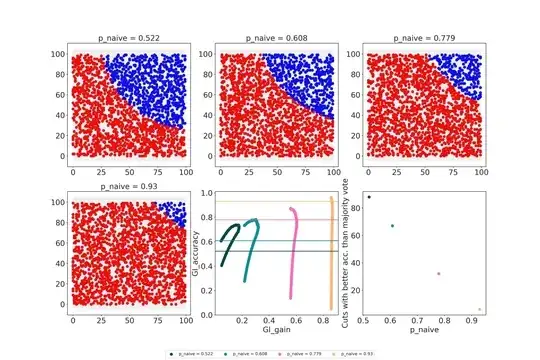
1. I have generated 4 x 2000 data points with random x/y coordinates.
2. Based on whether the result of np.sqrt((data.p_x*data.p_y)) was bigger or smaller than a cutoff, I have assigned either blue or red as colors.
3. Then, for each set of 2000 points, I have drawn 100 vertical lines representing potential splits a decision tree node could evaluate.
4. Then, for each of these splits, I followed the procedure described in https://victorzhou.com/blog/gini-impurity/#example-1-the-whole-dataset. So I basically evaluated the Gini Impurity for both sides of the split, then calculated a weighted sum of these per split and calculated the "Gini Gain" by subtracting that from the naive probability of being right.
5. In the lower-center plot, I have plotted the gain for each of these splits against the ratio of correct points this split would be able to classify. Also, for each set I have added a horizontal line indicating the number of correctly classified points if I just were to go for majority voting.

I simplified the real world by only using vertical splits, shown in light grey. Also, I'm approaching a 2D problem basically in 1D. The horizontal lines correspond be the accuracy of the majority vote principle you proposed.

I uploaded the code here: https://github.com/dazim/stackoverflow_answers/blob/main/gini-impurity-in-decision-tree-reasons-to-use-it.ipynb

Edit 2021-02-19:

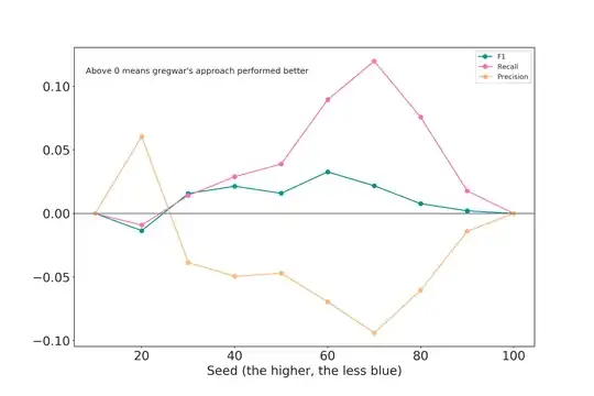
Based on the discussion in the comments I replaced the GI with the approach that Gregwar proposed. Based on the two approaches, I evaluated the performance of a node making the decision based on the best cut. Plotted is score_gregwar - score_GI Sadly, I've got to work on other stuff. But maybe someone else want's to pick up on that. Based on what I see in this simulation, the differences don't seem that big. However, using more "real" data and not just drawing vertical splits might change this. Sorry!