I am trying to implement bilinear interpolation as described in the paper Spatial Tranformer Networks by Jaderberg et. al (see link to paper). They describe bilinear interpolation in Equation 5 as:
$$ V_i^c = \sum_{n}^{H}\sum_{m}^{W} U_{nm}^c \max(0,1-|x_i^s - m|)\cdot\max(0,1-|y_i^s - n|), $$ where:
- $V_i^c$ is the resulting pixel value in the new image
- $H$ and $W$ are the height and width of the original image (or feature map) in pixels
- $c$ refers to the channel (e.g. RGB)
- $(x_i^s, y_i^s)$ are the coordinates where the original image is sampled (where the image is normalized such that $-1 \le x_i^s, y_i^s\le 1$)
- $U_{nm}^c$ is defined as the pixel value at location $(n,m)$ in channel $c$.
I am having trouble interpreting the variables $n$ and $m$. Are these
- coordinates in the normalized image (i.e. $-1 \le n, m\le 1$, where you would sum $n$ from $n=-1$ to $H=1$ in steps of the normalized resolution, e.g. steps of $1/100$ for an image that is 100 px in height)
- or are these row and column values (e.g. you sum $n$ from $n=0$ to $n=100$ for an image that is 100px in height)?
I have tried out both to do downsampling of an image, but don't get consistent results.
If someone can help me out interpreting this, I would appreciate it very much.
Below I have included what I understand of bilinear interpolation. Maybe that someone can help me out based on this.
In the below figure, a single channel feature map (or image) with one channel is displayed that consists of four pixels with values $ U_{nm} $, where $ n $ and $ m $ are the coordinates of the center of the pixels, i.e. $ m,n \in \{-0.5, 0.5\} $. If we index $ m $ and $ n $ as $ m_k, n_k $, with $ k \in [1,4] $, we can also index the pixel values as $ U_{n_km_k} $. The values of all four pixels can be reduced to a single value $ V $ at position $ (x_i^s, y_i^s) $ by applying bilinear interpolation.
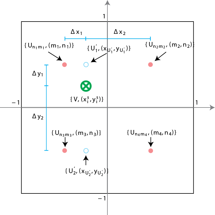
The procedure can be divided into three linear interpolations. First the value $ U_1' $ at position $ (x_{U_1'}, y_{U_1'}) $ can be computed by interpolating the values $ U_{n_1m_1} $ and $ U_{n_2m_2} $: \begin{equation} U_1' = \Delta x_2\ U_{n_1m_1} + \Delta x_1\ U_{n_2m_2}. \end{equation} As the sum of $ \Delta x_1 $ and $ \Delta x_2 $ is equal to one, due to normalization of the axes, the above equation can be rewritten as: \begin{equation} U_1' = (1-\Delta x_1) U_{n_1m_1} + (1-\Delta x_2) U_{n_2m_2}. \end{equation} The terms $ \Delta x_1 $ and $ \Delta x_2 $ can be expressed as: \begin{align} \Delta x_1 = |x_i^s - {m_1}|\\ \Delta x_2 = |x_i^s - {m_2}|, \end{align} which, substituted into the equation for $U_1'$ yields: \begin{equation} U_1' = U_{n_1m_1}(1-|x_i^s - {m_1}|) + U_{n_2m_2}(1-|x_i^s - {m_2}|). \end{equation}
Similarly the value for $ U_2' $ can be computed: \begin{equation} U_2' = U_{n_3m_3}(1-|x_i^s - {m_3}|) + U_{n_4m_4}(1-|x_i^s - {m_4}|). \end{equation}
Once $ U_1' $ and $ U_2' $ have been computed, $ V $ can be determined by linearly interpolating $ U_1' $ and $ U_2' $: \begin{equation} V = U_1'(1-\Delta y_1) + U_2'(1-\Delta y_2) . \end{equation} The values for $ \Delta y_1 $ and $ \Delta y_2 $ can be expressed as follows: \begin{align} \Delta y_1 = |y_i^s - y_{U_1'}| = |y_i^s - {n_1}| = |y_i^s - {n_2}|\\ \Delta y_2 = |y_i^s - y_{U_2'}| = |y_i^s - {n_3}| = |y_i^s - {n_4}| . \end{align}
Substituting the above equations and those of $\Delta x_1$ and $\Delta x_2$ into the equation for $V$ yields: \begin{equation} \begin{split} V &= U_{n_1m_1}\cdot (1-|x_i^s - {m_1}|) \cdot (1-|y_i^s - {n_1}|) \\ &+ U_{n_2m_2}\cdot (1-|x_i^s - {m_2}|) \cdot (1-|y_i^s - {n_2}|) \\ &+ U_{n_3m_3}\cdot (1-|x_i^s - {m_3}|) \cdot (1-|y_i^s - {n_3}|) \\ &+ U_{n_4m_4}\cdot (1-|x_i^s - {m_4}|) \cdot (1-|y_i^s - {n_4}|), \end{split} \end{equation} which can be written more compactly as: \begin{equation} \begin{split} V &= \sum_{k=1}^{4} U_{n_km_k} \cdot (1-|x_i^s - {m_k}|) \cdot (1-|y_i^s - {n_k}|)\\ &=\sum_{n}^{H}\sum_{m}^{W} U_{nm} \cdot (1-|x_i^s - {m}|) \cdot (1-|y_i^s - {n}|). \end{split} \end{equation}
Edit to clarify my comment to @D.W.
Initially I also thought that $n$ and $m$ are row and column indices as you normally do a summation over integer values. Also the summation is up to $H$ and $W$, respectively, which are the # of rows and # of columns. So it seems logical to think that $\sum_{n=1}^{H = \#rows}\sum_{m=1}^{W = \#columns}$, with $n=1,2,3,...,H $ and $m=1,2,3,...,W$.
However, when you apply it in this way, the terms within the summation will always be zero. This is because of the condition $-1 \le x_i^s, y_i^s \le 1$. Taking the example in the figure where $(x_i^s, y_i^s) = (-0,25, 0,25)$, we have: \begin{equation} \begin{split} V &= \sum_{n}^{H}\sum_{m}^{W} U_{nm}\cdot \max(0, 1-|x_i^s-m|)\cdot \max(0, 1-|y_i^s-n|) \\ &= U_{11}\cdot \max(0, 1-|-0.25-1|)\cdot \max(0, 1-|0.25-1|)\\ &+ U_{12}\cdot \max(0, 1-|-0.25-2|)\cdot \max(0, 1-|0.25-1|)\\ &+ U_{21}\cdot \max(0, 1-|-0.25-1|)\cdot \max(0, 1-|0.25-2|)\\ &+ U_{22}\cdot \max(0, 1-|-0.25-2|)\cdot \max(0, 1-|0.25-2|)\\ &= U_{11}\cdot 0 + U_{12}\cdot 0 + U_{21}\cdot 0 + U_{22}\cdot 0= 0 \end{split} \end{equation} When you have $n$ go from $n=0$ to $H-1$ (and similarly for $m$), it does work in this (simple) example, which would lead to concluding that $n$ and $m$ should start from zero.
However, when you try to apply this to an image which is larger than 2x2 pixels, you get a similar problem than the one for $n=1, ..., H$, i.e. all elements within the summation will be zero when $n>0$ and $m>0$.
To clarify this, look at the below image. Here the original image is an 8x8 image with pixels depicted by black squares. We wish to downsample the image to a 6x6 image, depicted by the dashed red squares. If we want to compute the value of the pixel marked by the pink star with coordinates $(x_1^s, y_1^s) = (-0.833, 0.833)$, we would have: \begin{equation} \begin{split} V_{1} &= \sum_{n}^{H}\sum_{m}^{W} U_{nm}\cdot \max(0, 1-|x_1^s-m|)\cdot \max(0, 1-|y_1^s-n|) \\ &= U_{00}\cdot \max(0, 1-|-0.833-0|)\cdot \max(0, 1-|0.833-0|)\\ &+ U_{01}\cdot \max(0, 1-|-0.833-1|)\cdot \max(0, 1-|0.833-0|)\\ &+ U_{02}\cdot \max(0, 1-|-0.833-2|)\cdot \max(0, 1-|0.833-0|)\\ &+ ...\\ &+ U_{10}\cdot \max(0, 1-|-0.833-0|)\cdot \max(0, 1-|0.833-1|)\\ &+ U_{11}\cdot \max(0, 1-|-0.833-1|)\cdot \max(0, 1-|0.833-1|)\\ &+ ...\\ &+ U_{77}\cdot \max(0, 1-|-0.833-7|)\cdot \max(0, 1-|0.833-7|)\\ &= U_{00}\cdot 0.167^2 + U_{10}\cdot 0.167\cdot 0.833, \end{split} \end{equation} which is only a function of $U_{00}$ and $U_{10}$ and not of $U_{00}$, $U_{01}$, $U_{10}$ and $U_{11}$ as one would reason.
If we look at the blue star with coordinates $(x_{49}^s, y_{49}^s) = (0.833, -0.833)$ and apply the same equation, we have: \begin{equation} \begin{split} V_{49} &= \sum_{n}^{H}\sum_{m}^{W} U_{nm}\cdot \max(0, 1-|x_{49}^s-m|)\cdot \max(0, 1-|y_{49}^s-n|) \\ &= U_{00}\cdot \max(0, 1-|0.833-0|)\cdot \max(0, 1-|-0.833-0|)\\ &+ U_{01}\cdot \max(0, 1-|0.833-1|)\cdot \max(0, 1-|-0.833-0|)\\ &+ U_{02}\cdot \max(0, 1-|0.833-2|)\cdot \max(0, 1-|-0.833-0|)\\ &+ ...\\ &+ U_{10}\cdot \max(0, 1-|0.833-0|)\cdot \max(0, 1-|-0.833-1|)\\ &+ U_{11}\cdot \max(0, 1-|0.833-1|)\cdot \max(0, 1-|-0.833-1|)\\ &+ ...\\ &+ U_{77}\cdot \max(0, 1-|0.833-7|)\cdot \max(0, 1-|-0.833-7|)\\ &= U_{00}\cdot 0.167^2 + U_{01}\cdot 0.833\cdot 0.167, \end{split} \end{equation} which again is only function of $U_{00}$ and $U_{01}$ and not of $U_{66}$, $U_{67}$, $U_{76}$ and $U_{77}$ as one would expect.
I have also tried normalizing $n$ and $m$, such that $n =-1, -1+ 2/8, -1 +4/8, ..., 1$ (and similarly for $m$, but I end up with similar problems.
